rpwf • rpwf

Introduction

I wrote this package because I want to wrangle data in R, i.e., using data.table, tidymodels, tidyverse, spline basis functions generations with mgcv/gratia, and visualization with ggplot2 to name a few.
- Importantly, mice and missForest in R are powerful imputation methods.
Meanwhile, the ML and DL ecosystem in python can be more mature and many latest updates and research papers only have python implementations.
- I find that fitting a model in python can be faster and consume less memory for the equivalent model in R, possibly due to numpy and bleeding edge implementations.
rpwf allows wrangling data in R while having access to the latest and greatest ML packages in python.
In Kaggle competitions, it is usually feature engineering that gives a competitor an edge. rpwf helps by
- Enabling the use of the workflowset framework. Workflow sets can be used as pre-defined test experiments that test how engineered features affect a model’s predictive performance.
- Allowing seamless deployment on HPC clusters or cloud computers because the pathing and uploading of results is handled by (a) SQLite database(s) and the pins package.

Demonstration

library(rpwf)
library(dplyr)
library(parsnip)
library(recipes)
library(ggplot2)
library(pins)

Let’s demonstrate using the sim_classification() function from modeldata.

set.seed(123)
tmp_dir <- tempdir() # Temp folder
df <- modeldata::sim_classification(num_samples = 500, num_linear = 40)
df[1:6, 1:6]
#> # A tibble: 6 × 6
#>   class   two_factor_1 two_factor_2 non_linear_1 non_linear_2 non_linear_3
#>   <fct>          <dbl>        <dbl>        <dbl>        <dbl>        <dbl>
#> 1 class_2       -0.364       -1.08       -0.681         0.854        0.206
#> 2 class_2        0.292       -0.884      -0.711         0.666        0.943
#> 3 class_1        1.39         2.61       -0.702         0.733        0.379
#> 4 class_2       -0.354        0.535       0.0289        0.315        0.626
#> 5 class_2        1.06        -0.727      -0.0143        0.668        0.184
#> 6 class_1        2.26         2.15        0.233         0.464        0.659

Data is balanced.

table(df$class)
#> 
#> class_1 class_2 
#>     228     272

There’s no missing data.

sum(is.na(df))
#> [1] 0

Re-code class, our response variable, as integers

df$class <- as.integer(df$class) - 1L

Add an optional id column

df$id <- seq_len(nrow(df))

Initialize a database

Create a pins::board_<board type> and pass it to rpwf_connect_db().
Create a database called "db.SQLite" with rpwf_connect_db().

board <- board_temp()
db_con <- rpwf_connect_db(paste(tmp_dir, "db.SQLite", sep = "/"), board)

db_con is an object that holds a DBI connection to the SQLite database that was just created. Access it with db_con$con.

db_con$con
#   Path: <path>/rpwfDb/db.SQLite
#   Extensions: TRUE

Define models with parsnip

Identical to {parsnips}, first choose a model, i.e., boost_tree(), then choose the R engine with set_engine() and classification or regression with set_mode().
Then, pipe the object into the set_py_engine() function.
set_py_engine() has 3 important parameters
- py_module and py_base_learner defines how to import a base learner in a python script.
- tag is an optional parameter that’s helpful for keeping track of models.
- Arguments passed to the base learner in python can be passed to ... of set_py_engine()
Check the available models with rpwf_avail_models() and add another model with rpwf_add_py_model().

rpwf_avail_models(db_con) |> head()
#>              py_module    py_base_learner r_engine     model_mode
#> 1 sklearn.linear_model LogisticRegression   glmnet classification
#> 2 sklearn.linear_model         ElasticNet   glmnet     regression
#> 3          sklearn.svm                SVC  kernlab classification
#> 4          sklearn.svm                SVR  kernlab     regression
#> 5              xgboost      XGBClassifier  xgboost classification

`xgboost`

I fix the n_estimators at 50 and tune the learning rate. Other arguments can be found at the xgboost docs.
To do this, I pass the argument n_estimators = 50 to set_py_engine().
I am going to tune 6 hyper parameters by passing them the tune() functions just like in {parsnips}.

# This model is equivalent to the following python codes:

# from xgboost import XGBClassifier
#
# base_learner = XGBClassifier(
#   eval_metric = "logloss",
#   use_label_encoder = False,
#   verbosity = 0,
#   silent = True
# )

xgb_model <- boost_tree(
  mtry = tune(),
  min_n = tune(),
  tree_depth = tune(),
  learn_rate = tune(),
  loss_reduction = tune(),
  sample_size = tune()
) |>
  set_engine("xgboost") |>
  set_mode("classification") |>
  set_py_engine(
    "xgboost",
    "XGBClassifier",
    rpwf_model_tag = "xgboost",
    eval_metric = "logloss",
    n_estimators = 50,
    use_label_encoder = FALSE,
    verbosity = 0,
    silent = TRUE
  )

`svm`

From the sklearn.svm.SCV docs, the parameter cache_size can help speed up model fitting if memory is available. I will increase this from the default value. This is an example of how fitting models in python can have some very useful settings.
- In this example, cache_size wouldn’t reduce fit time because the data is small.
Let’s set up a radial basis kernel svm model.
- I have to fix the kernel parameter as rbf.
- This is because tidymodels defines svm_poly() and svm_rbf() separately for polynomial basis svm and radial basis svm while sklearn.svm.SVC defines them both with the kernel parameter.

svm_rbf_model <- svm_rbf(
  cost = tune(),
  rbf_sigma = tune()
) |>
  set_engine("kernlab") |>
  set_mode("classification") |>
  set_py_engine(
    "sklearn.svm",
    "SVC",
    rpwf_model_tag = "svm_rbf",
    kernel = "rbf", # fix kernel parameter = "rbf"
    cache_size = 500
  )

`glm`

Let’s also fit an elastic net model.

enet_model <- logistic_reg(
  penalty = tune(),
  mixture = tune()
) |>
  set_engine("glmnet") |>
  set_mode("classification") |>
  set_py_engine(
    "sklearn.linear_model",
    "LogisticRegression",
    rpwf_model_tag = "glmnet",
    solver = "saga",
    penalty = "elasticnet",
    max_iter = 1000
  )

Hyper parameter tuning

The dials package provides
1. sensible hyper parameters ranges
2. functions that go beyond the random grid and regular grid such as dials::grid_max_entropy(), and dials::grid_latin_hypercube().
dials::grid_latin_hypercube() will be helpful for models with a lot of hyper parameters such as xgboost. But for svm_rbf_model, tuning just 2 hyper parameters on a 2-D grid with dials::grid_regular() would provide sufficient coverage of the hyper parameter space at an acceptable speed.
Updating the range of the hyper parameter space is similar to how it works in dials. Just provide the tuning functions (or create new ones) to the hyper_par_fun parameter.
Models specific tuning grids can be added at this step with set_r_grid().

`xgboost`

For the xgboost_model, let’s use a dials::grid_latin_hypercube().
Let’s limit max_depth. To do this, I add a named list to the hyper_par_fun parameter.

xgb_model <- xgb_model |>
  set_r_grid(
    grid_fun = dials::grid_latin_hypercube,
    hyper_par_fun = list(tree_depth = dials::tree_depth(range(2, 5))),
    size = 100
  )

`svm`

For the svm_rbf_model, let’s use a 2D regular grid.

svm_rbf_model <- svm_rbf_model |>
  set_r_grid(dials::grid_regular, levels = 10)

`glm`

Let’s also use a 2D regular grid for the enet model. However, I changed the range of the l1 penalty to allows for a greater regularization strength since scikit-learn inverse the penalty value for the logistic regression implementation.

enet_model <- enet_model |>
  set_r_grid(dials::grid_regular,
    list(penalty = dials::penalty(range = c(-8, 0.5))),
    levels = 10
  )

Define transformation pipelines with recipes

Recipes are defined as usual.
- Use the formula or the role interface to specify the response and predictors.
- The base recipe is used to gauge the baseline performance of each model.
- The pca recipe is used to de-correlate the variables. step_pca() conveniently provides a parameter to keep an arbitrary threshold of the variance explained. I choose 95%.
rpwf reserves one optional special role that can be used with the update_role() function:
- pd.index is a special role. It will mark a column for conversion into a pandas index in python.
- Below, the column df$id will become the pandas.DataFrame index.
Pipe a recipe into rpwf_tag_recipe() to add a description to the recipe.

common <- recipe(class ~ ., data = df) |>
  step_mutate(class = as.integer(class)) |>
  update_role(id, new_role = "pd.index")

### xgb recipes
xgb_base_rec <- common |>
  rpwf_tag_recipe("xgb_base")

xgb_pca_rec <- xgb_base_rec |>
  step_normalize(all_numeric_predictors()) |>
  step_pca(threshold = .95) |>
  rpwf_tag_recipe("xgb_pca")

### glm and svm recipes
scaled_base_rec <- common |>
  step_normalize(all_numeric_predictors()) |>
  rpwf_tag_recipe("scaled_base")

scaled_pca_rec <- scaled_base_rec |>
  step_pca(threshold = .95) |>
  rpwf_tag_recipe("scaled_pca")

Create workflowsets

`rpwf_workflow_set()`

The function rpwf_workflow_set() mimics workflowsets::workflow_set(). It creates a combination of all the provided recipes and models. Then, one can work with the resulting data.frame just like any data.frame (e.g., filtering out redundant workflows and etc.).
One workflow_set for xgboost and one for svm and glm are created and rbind() into one final workflow_set.
The cost parameter is to specify which measure of predictive performance is optimized for. Look up the values in the scikit-learn docs. Custom cost functions are possible but would require coding on the python side.

### xgboost workflow_set
xgb_wfs <- rpwf_workflow_set(
  preprocs = list(xgb_base_rec, xgb_pca_rec),
  models = list(xgb_model),
  cost = "roc_auc"
)

### svm and glm workflow_set
svm_glm_wfs <- rpwf_workflow_set(
  preprocs = list(scaled_base_rec, scaled_pca_rec),
  models = list(svm_rbf_model, enet_model),
  cost = "roc_auc"
)

### combined workflow_set
all_wfs <- rbind(xgb_wfs, svm_glm_wfs)

`rpwf_augment()`

rpwf_augment() is a wrapper function for many tasks. But most importantly, it generates the hyper parameter grids in R and transform these grids to make them compatible with sklearn’s API. For example the following conversions were done:
- The mtry positive integer in R is converted into sklearn’s colsample_bytree positive proportions.
- The penalty in R is reciprocated in sklearn logistic regression. This is why in order to have the l1 penalty > 1 (which is too large most of the time), the range upper bound is changed to be positive and smaller than 1.

all_wfs <- rpwf_augment(all_wfs, db_con)
all_wfs |>
  dplyr::select(model_tag, recipe_tag, costs)
#> # A tibble: 6 × 3
#>   model_tag recipe_tag  costs  
#>   <chr>     <chr>       <chr>  
#> 1 xgboost   xgb_base    roc_auc
#> 2 xgboost   xgb_pca     roc_auc
#> 3 svm_rbf   scaled_base roc_auc
#> 4 glmnet    scaled_base roc_auc
#> 5 svm_rbf   scaled_pca  roc_auc
#> 6 glmnet    scaled_pca  roc_auc

Checking the generated grids, we can see that the names of the hyper parameters have been renamed to conform to the scikit-learn API.

sapply(unique(all_wfs$grids), head)
#> [[1]]
#> # A tibble: 6 × 6
#>   colsample_bytree min_child_weight max_depth learning_rate        gamma subsa…¹
#>              <dbl>            <int>     <int>         <dbl>        <dbl>   <dbl>
#> 1            0.533                7         5       0.00437      2.51e-2   0.478
#> 2            0.244               31         4       0.191        1.69e-9   0.835
#> 3            0.511                7         4       0.260        2.23e-8   0.996
#> 4            0.733               20         2       0.0257       5.94e-4   0.225
#> 5            0.711               32         4       0.00658      1.46e+0   0.309
#> 6            0.911                3         4       0.00111      9.41e-7   0.642
#> # … with abbreviated variable name ¹subsample
#> 
#> [[2]]
#> # A tibble: 6 × 2
#>         C   gamma
#>     <dbl>   <dbl>
#> 1 1024    0.00862
#> 2  323.   0.00862
#> 3  102.   0.00862
#> 4   32    0.00862
#> 5   10.1  0.00862
#> 6    3.17 0.00862
#> 
#> [[3]]
#> # A tibble: 6 × 2
#>            C l1_ratio
#>        <dbl>    <dbl>
#> 1 100000000      0.05
#> 2  11364637.     0.05
#> 3   1291550.     0.05
#> 4    146780.     0.05
#> 5     16681.     0.05
#> 6      1896.     0.05

Here are the dimensions of the grids. This is always good to check to make sure we didn’t accidentally make a grid that’s too big.

sapply(unique(all_wfs$grids), nrow)
#> [1] 100 100 100

Export data as parquets and add to database.

There are two types of parquets files: 1) hyper param grids, and 2) train/test data.
rpwf_write_grid() and rpwf_write_df() write the parquets.
Because this function only generate a data.frame if its not already written, running each of these functions in parallel is not recommended.
- To get around this, one can either work with a manageable number of workflows at a time, or split the work into multiple different databases and run the export functions in parallel over the databases.

rpwf_write_grid(all_wfs)
rpwf_write_df(all_wfs)

Export the board information as a YAML file.
Then finally, export the meta data into the database with rpwf_export_db().

rpwf_write_board_yaml(board, paste(tmp_dir, "board.yml", sep = "/"))
rpwf_export_db(all_wfs, db_con)
#> [1] 6

Run the workflow in python

The rpwf python codes contains scripts that performs model fitting. These are also templates to experiment further using the data generated in R.
For example, to use the nested_resampling.py script, in the terminal, run the following command to get the list of arguments

python -m rpwf.script.nested_resampling -h

Or the following in a Jupyter notebook cell

%run -m rpwf.script.nested_resampling -h

This following command display the workflows we exported.

%run -m rpwf.script.nested_resampling $<path to the db> -b $<path to board yaml> -s

The positional argument is the path to the database.
The -b flag is the path to the exported board YAML file associated with this db.
The -s flag shows the workflows present in the database.
The other important flags are
- The -a flag runs all the workflow that hasn’t been run.
- The -w flag accept a list of ids (i.e., 1 2 3 4) to specify which workflow to run.
- The -f flag force a run and overwrite the results of a workflow that has already been run.
- The -c flag indicates the number of CPU cores dedicated to the model fitting task.
- The -icv and -icr flags are number of vfold-cv and repeats for the inner loop used for hyper parameters tuning.
- The -ocv and -ocr flags are number of vfold-cv and repeats for the outer loop used for testing the predictive performance.
Let’s run the nested CV with 5 CV * 2 repeats for the inner loop and 5 CV * 2 repeats on the outer loop.

%run -m rpwf.script.nested_resampling $<path to the db> -b $<path to board yaml> \
  -a -c 7 -icv 5 -icr 2 -ocv 5 -ocr 2

Visualize the results

Results can be imported back into R by passing the db_con object to rpwf_results().

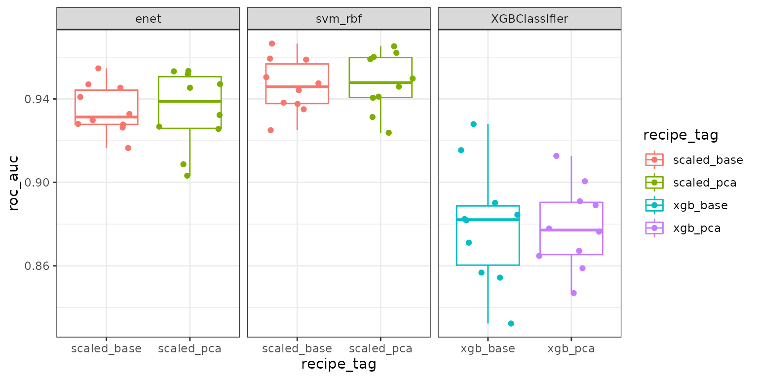
fit_results <- rpwf_results(db_con)

We can now just manipulate the results with R.

fit_results |>
  tidyr::unnest(fit_results) |>
  ggplot(aes(y = roc_auc, x = recipe_tag, color = recipe_tag)) +
  geom_boxplot() +
  geom_jitter() +
  facet_wrap(~model_tag, scale = "free_x") +
  theme_bw()